
English edition of the exploratory research paper. Editorial date: 24 October 2026.
Keywords AI inference economics · Token Deflation Trap · accelerated computing · price elasticity of demand · commercial life of compute · cost per accepted task · net present value · Saudi Arabia
In this article
The Token Deflation Trap: A Reproducible Synthetic Study of the Commercial Life of Accelerated AI Compute
Work status: Owner-review draft. Model actually executed on synthetic data, with no original financial or operational data from a Saudi facility. Version: 1.0 | Not peer reviewed.
Extended abstract
Background: AI chips and inference-serving software are advancing rapidly, while investment in AI infrastructure is consumed over relatively long contractual and accounting periods. Conflating improvements in physical productivity, the cost of producing a token, its selling price, and the use of billable capacity leads to conflicting conclusions about capital viability. Question: Under what conditions does software efficiency improve the economic return on accelerated-computing investment, and under what conditions does demand rebound fail to offset price decline? Method: A focused review of original disclosures and inference technologies, together with an implemented six-year discounted cash-flow (DCF) model using three hypothetical rates of price decline, three demand elasticities, and three rates of capacity improvement: 27 synthetic experiments in total, plus 18 additional sensitivity tests and a binary search for a conditional elasticity threshold. Calculated results: The experiments comprise 12 positive and 15 negative net present value (NPV) cases. The hypothetical reference case produces −5.58 accounting units despite reaching nominal payback during year five, and the demand-elasticity threshold required to cross zero in this case is approximately 0.7803. If variable unit cost is held constant instead of improving, the value becomes −31.18. Interpretation: These numbers do not represent prevalence, probability, or company returns. They expose the logic through which demand, capacity, cost, and discounting interact under stated assumptions. Methodological conclusion: Testing Saudi computing investments requires data on quality-accepted tasks, full delivery cost, actual contracts, and commercial life by workload. Processor count, utilization, or laboratory performance alone is insufficient.
Keywords: computational economics; graphics processing units (GPU); Token Deflation Trap; demand price elasticity; inference serving; cost per accepted task; net present value (NPV); Saudi Arabia.
English Abstract
Background: Accelerated AI hardware has multiple competing lifetimes: physical operability, accounting depreciation, contractual commitment, software relevance, and commercial advantage. Hardware efficiency gains do not automatically translate into increased revenue or positive investment returns. Objective: To identify conditional mechanisms through which declining billed inference-unit prices, demand elasticity, and effective capacity growth jointly determine a stylized investment's discounted cash flows. Methods: We examined a bounded set of primary technical and financial records listed in the reference register and executed a fully synthetic six-year cash-flow model with 27 factorial scenarios, 18 additional sensitivities, and a binary-search break-even elasticity calculation. Results: Twelve deliberately constructed scenarios yielded positive net present value and fifteen negative values. An illustrative base case yielded NPV −5.58 index units despite nominal payback in year five. The conditional break-even elasticity was approximately 0.7803. Holding unit variable cost fixed in the base case lowered NPV to −31.18. Interpretation: These figures are mathematical implications of chosen assumptions, not statistical estimates, observed Saudi outcomes, estimates of CoreWeave's profitability, or predictions for 2030. The central testable conjecture is that quality-adjusted, billable inference demand and realized unit margins, rather than installed accelerator count or standalone benchmark scores, more directly determine recoverable computing capital. Next study: A privacy-preserving, preregistered-in-advance panel of heterogeneous workloads and hardware vintages is proposed, with production billing and accepted-task outcomes.
Keywords: AI inference economics; accelerated computing; price elasticity; economic obsolescence; NPV; throughput; memory caching; Saudi Arabia.
1. Scientific question and boundaries
This paper examines an investment unit in AI computing capacity whose capacity can be rented or sold as services, not the Saudi economy as a whole. The unit can represent a collection of hardware and an inference service within a specified capital-expenditure (Capex) limit, but it does not represent an actual data center or a particular processor model. Its importance is methodological: how do we distinguish the path on which a technical improvement raises revenue margin from one on which output rises but capital recovery weakens?
The principal question is: if the realized price per unit of work declines, how do demand elasticity, effective capacity, variable cost, and cash-flow timing interact to determine the present value of a fixed initial investment? Five questions follow:
- Is a lower token price sufficient evidence that the cost of delivering a task has fallen?
- At what point does additional demand produce billable units, and at what point is it blocked by capacity, quality, or response-time limits?
- Can better software make an existing device more profitable even as price declines?
- How sensitive is the investment result to variable cost and the discount rate, rather than nominal capacity alone?
- Which public and authorized Saudi data could test these relationships without exposing operating load or contractor secrets?
The original unit of analysis proposed for a future application is a workload class × hardware vintage pair. When these pairs are combined in an aggregate statistic, the workload distribution should be disclosed rather than reduced to an average detached from the type of service.
2. Separating five lifetimes that are often conflated
We distinguish physical life, during which hardware remains operable; accounting useful life, which determines depreciation; contractual coverage, during which parties commit to pay for capacity; workload-adjusted technical life, during which a platform can perform specified workloads within quality and time requirements; and commercially advantageous life, during which it can compete against alternatives at prices that produce an adequate margin.
This separation is neither an official classification approved by a Saudi authority nor a general estimate of the computing market. It is a proposed analytical definition for comparing assets with different lifetimes. CoreWeave’s annual report illustrates why separation is necessary. The company changed the estimated useful life of its computing equipment from five years to six, effective January 2023, attributing the change to advances in hardware and software and data-center design. It also disclosed committed contracts with a weighted average term of about five years at the end of 2025 S01. Subtracting one number from the other to calculate a “year of profit” would be invalid: a contract does not equal a single asset cohort, and a weighted duration is not the expiry date of every obligation.
In 2026, NVIDIA introduced Rubin with claims of inference costs up to ten times lower than Blackwell under reference-workload designs. In September, OpenAI announced prices for newer API products that were lower than earlier products in the comparison class S03S04. The first is a promotional benchmark cost from a hardware manufacturer. The second is published selling prices from a service provider. A possible third measure, which we did not observe, is the price actually realized after contracts, discounts, and usage. Moving from one to another is an error in defining the variable, not a difference of opinion.
3. Technical literature: why value emerges between memory and the queue
Realized productivity depends on more than peak compute, and on techniques whose benefit can increase without replacing every hardware component:
Memory management: PagedAttention and vLLM, in Kwon et al. (2023), use partitioning and reuse of key-value cache (KV cache) memory to reduce internal fragmentation and unused reservation. The paper’s experiments reported throughput roughly two to four times that of specified baselines at similar latency S05. Reproducing that ratio in Saudi Arabia would require platform, workload, and version specifications; the paper does not support a direct commercial generalization.
Scheduling: Orca (2022) proposed iteration-level scheduling to reduce short requests being blocked behind long ones and to apply selective batching S06. It is a reminder that waiting time can arise from a software decision as much as from processor capacity.
Disaggregating inference phases: TensorRT-LLM’s technical documentation distinguishes prefill from decode and explains why each phase may suit a different allocation of resources and parallelism. It also identifies the cost of moving the inference cache under disaggregation, so the approach is neither free nor best for every request S07.
Benchmark point: In September 2026, MLCommons announced MLPerf Inference v6.1, including benchmarks for multistep tasks S11. Its results can help establish standardized performance baselines, but they are not NPV or a commercial comparison after electricity, financing, and sales terms.
The paper derives a possible mechanism, not causal proof. When scheduling, memory management, and computational phases improve, an existing asset can produce more services. How much of that increase is billed depends on demand, customer behavior, output quality, and competitive conditions. The gain may accrue to the computing operator, application developer, end user, or be divided among them.
4. Competing hypotheses
- H1, capacity effect: When capacity is the constraint and paid demand can absorb additional output, an increase in deliverable capacity raises net value, provided expansion and operating costs do not overwhelm it.
- H2, price-deflation effect: With inelastic demand, revenue may fall quickly despite an increase in units, making payback harder within a specified financing horizon.
- H3, decisive rebound: When demand is highly elastic and capacity exists to meet it, total revenue may rise after a price decline. This is not a judgment that operating profit must rise.
- H4, contract versus spot market: When multiyear capacity-purchase commitments exist, forward revenue has a different exposure to the spot service price. Delivery rights, default, concessions, and renewal make that protection conditional.
- Competing hypothesis R1: Compute abundance may produce lower unit prices alongside strong profitable growth because new high-value uses absorb capacity. In that case the trap will not appear in realized-profit data.
- Null hypothesis H0: After controlling for workload mix, electricity, financing, contracts, and quality, the rate of unit-price decline has no additional explanatory power for investment return. This hypothesis should not be rejected without actual operating data and an appropriate causal-inference design.
These are hypotheses and interpretive propositions. Our computational tests examine their consistency inside a model built from assumptions; they do not test them on people or actual facilities.
5. Implemented model design and units
Inputs and notation: For each year t = 1,...,6, p0 denotes an initial price index of 1, q0 annual demand of 50 units, k0 deliverable annual capacity of 50, c0 initial variable cost per unit of 0.20, F annual fixed operating cost of 7, I0 an initial investment of 120, S an assumed residual value of 8 at the end of year six, and r a discount rate of 12%. These are all hypothetical index units. They do not denote dollars, riyals, megawatts, devices, or real tokens.
The tested variables are δ, the annual rate of decline in unit price; ε, the absolute value of price elasticity of demand; and g, the rate at which saleable capacity improves through an operating improvement assumed to persist. The following formulas were implemented in code:
D_t is potential demand, K_t the ceiling on qualified service, X_t billable units, and CF_t operating cash flow with residual value in the final year. We assumed that one transaction or request equals one unit and that every delivered unit meets quality and service requirements. This is a convenient and not necessarily realistic assumption that would need to be separated empirically. The minimum function prevents revenue from being modeled for demand that finds no capacity. The model does not include debt, interest, tax, wage changes, accounting depreciation, counterparty failure, or hardware outages. The cost of capital is represented by an assumed discount rate, not a loan price inferred from an American filing.
The assumption c_t = c0/(1+g)^(t-1) requires great caution. We assumed that software productivity lowers variable cost per unit at the same rate. This may fail if most of the improvement allows more workloads to run without actually reducing energy or network expense. We therefore implemented a sensitivity path that holds c_t at c0 regardless of capacity changes. The conservative result appears in Section 8.
6. Data, implementation, and reproducibility
The study contains no bank transaction record or utilization figure from a Saudi operator. Every experimental value comes from the readable data/model_assumptions.json; analysis/reproduce.py performs the calculations in Python using only the standard library. Execution produces five actual records:
base_annual_cashflows.csv: six rows for annual cash flow, volume, capacity, revenue, and discounting.synthetic_scenario_results.csv: a grid of 27 independent cases in a 3×3×3 design.sensitivity_checks.csv: 18 additional cases crossing three discount rates (8%, 12%, 16%), three rates of capacity improvement (0%, 25%, 50%), and two states in which variable cost either improves or remains fixed.derived_checks.json: a derived summary of the threshold, base result, and case counts.- Figures and charts in SVG and PNG generated from the resulting tables, not from estimated drawings.
A reviewable spreadsheet, evidence_workbook.xlsx, separates adjustable inputs from calculations and result images. It is an inspection aid; it does not replace the script as the published computational record of the full experiment. We used an annual forecast paid at year-end, an investment at time zero, and residual value in year six only. No external financial sources feed the synthetic numbers. External sources establish reasons to test the mechanisms and the limits on applying them to reality.
7. Results of the executed experiment: why demand does not always win
We executed a grid with annual price declines of 10%, 22%, or 35%; demand elasticities ε of 0.5, 1.0, or 1.8; and capacity growth rates of 0%, 25%, or 50%. Every combination produces six years and a present-value result. The values were neither randomly drawn nor used to estimate a probability distribution. The share of winning cases within the grid is therefore not an expected success rate in reality. It is a count of regions in a value space we selected.
Base case: annual price decline of 22%, elasticity of 0.7, annual capacity and unit-cost improvement of 25%, and a 12% discount rate. The annual results are calculated values, not editorial forecasts:
| Year | Price index | Potential demand | Available capacity | Units sold | Hypothetical revenue | Annual cash flow, including residual value where applicable |
|---|---|---|---|---|---|---|
| 1 | 1.000 | 50.00 | 50.00 | 50.00 | 50.00 | 33.00 |
| 2 | 0.780 | 59.50 | 62.50 | 59.50 | 46.41 | 29.89 |
| 3 | 0.608 | 70.80 | 78.13 | 70.80 | 43.08 | 27.01 |
| 4 | 0.475 | 84.25 | 97.66 | 84.25 | 39.98 | 24.35 |
| 5 | 0.370 | 100.25 | 122.07 | 100.25 | 37.11 | 21.90 |
| 6 | 0.289 | 119.30 | 152.59 | 119.30 | 34.44 | 27.63* |
Year six includes an assumed residual value of eight units. All columns contain synthetic index numbers rounded to two or three decimal places. The exact calculations are in the CSV.
Demand more than doubles even as annual revenue falls from 50 to about 34.44. Total revenue over six years is about 251.02 units, but revenue is not profit: variable and fixed costs and the timing of the investment leave NPV of about −5.5835. Cumulative cash flow after the initial cost becomes nonnegative in year five without discounting, while present value remains negative because money returning later carries less weight. Payback period must not be conflated with NPV.
The following selected comparison holds annual price decline at 22% and capacity improvement at 25%, changing elasticity only:
| Assumed demand elasticity | Six-year NPV in hypothetical units | Year-six revenue | Analytical result |
|---|---|---|---|
| 0.5 | −17.98 | 26.87 | Volume growth is insufficient to offset price deflation. |
| 1.0 | +8.91 | 44.05 | Higher demand fills saleable capacity. |
| 1.8 | +8.91 | 44.05 | The result is identical because the capacity ceiling constrains delivery. |
The equality of the 1.0 and 1.8 rows is not arbitrary rounding. In every year after the first under these assumptions, available demand exceeded billable capacity, so X_t = K_t; raising willingness to buy cannot change realized output. Growth in the potential market, deliverable volume, and actually paid volume must therefore be distinguished. If a service is unavailable at the same price, intense enthusiasm cannot compensate unless capacity can expand or price can rise within customer tolerance.
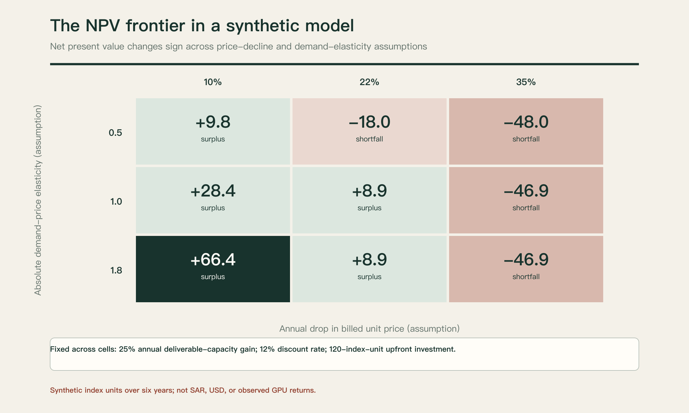
Figure 1: Matrix of results from an executed experiment over multiple elasticities and prices, with the assumption of 25% annual capacity improvement held fixed. The numbers are neither probability distributions nor estimates of Saudi institutions.
The full experiment produced 12 positive-NPV and 15 negative-NPV scenarios out of 27, with mixed signs along the three axes. When capacity is fixed at 50 units throughout the six years (g=0), every result under the selected settings is negative because demand rises but no more than fifty units can be delivered while price keeps falling. At the opposite extreme, one highly elastic, high-capacity scenario (δ=.22, ε=1.8, and g=.50) reaches about +113.75. That result depends on an extreme assumption of fast software-productivity growth over consecutive years; it is not an argument for actual investment using these numbers.
8. Sensitivity results and when the conclusion changes
We tested discount rates of 8%, 12%, and 16%; capacity improvements of 0%, 25%, and 50%; and variable unit cost either declining at the assumed rate or remaining constant. For the case of a 22% price decline and elasticity of 0.7, the following results appeared at 25% capacity improvement:
| Discount rate | Assumes variable cost improves with capacity | Assumes variable cost remains fixed |
|---|---|---|
| 8% | +7.84 | −22.46 |
| 12% | −5.58 | −31.18 |
| 16% | −16.82 | −38.62 |
Interpreting the results matters more than memorizing the values. Removing the assumption of declining variable unit cost makes capacity improvements alone insufficient to produce the assumed return, because revenue is determined by what demand buys rather than by what software can run. In some combinations, raising g from 25% to 50% no longer affects revenue after supply reaches required demand, so long as selling price and demand volume remain unchanged. This is not a rejection of software. It asks which constraint was actually removed: compute, cost, or the existence of a customer?
We used an iterative binary search over ε from 0 to 2.5, holding every other base-case value fixed, to find the lowest elasticity at which NPV≥0. It was approximately 0.7803. This is not an estimated elasticity for Saudi or global demand. It is a threshold within a particular model; changing initial investment, price, delivery quality, demand characteristics, or the discount period changes it. It can be recalculated by inspecting data/derived_checks.json and running the script, not by relying on a familiar economic label.
Limits of these tests: We did not examine random distributions of electricity increases, network congestion, contract loss, or data-center geography. We used no statistical samples, so there are no p values, confidence intervals, or claims of statistical significance. Nor do we claim that 18 tests represent the entire risk space. The tests cover three intersecting sets of specified and disclosed parameters.
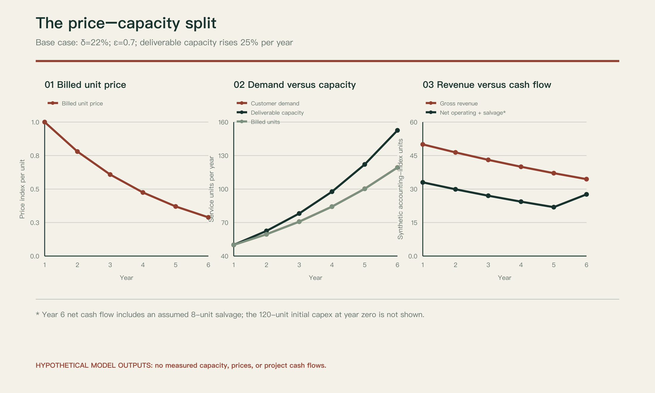
Figure 2: Base-case results. Capacity improvement, price aging, and cash-flow timing are different phenomena; the financial-axis unit is merely a synthetic index.
9. Testing relevance to Saudi Arabia without projecting one company’s data onto another
Three classes of original fact have empirical relevance, but they do not form a single measurement series:
A. An American commercial disclosure, not a Saudi measurement: CoreWeave’s 2025 report shows different accounting and contractual lives, while its 2026 statements report remaining performance obligations (RPO) of $103.7 billion at 30 June 2026, of which 41% was expected to be recognized in the first 24 months after that date, 39% in months 25–48, and the remainder through month 78 S01S02. The filing also gives total future debt-principal payments of $35.551 billion in a comprehensive maturity schedule S02. Adding or dividing the figures cannot establish a coverage ratio or support a conclusion of crisis or surplus. The first represents contractual services not yet provided under revenue-recognition rules; the second comprises financing obligations at different dates. They are not opposing net cash flows. Long-term contracts may insulate an operator from spot prices, but we did not analyze their individual terms or performance records.
B. A Saudi operating announcement from commercial parties: On 31 August 2026, AMD, Cisco, and HUMAIN announced that systems using AMD Instinct MI355X processors and Cisco Silicon One networking in Saudi Arabia had entered production to serve HUMAIN customers inside and outside the Kingdom S09. The same announcement disclosed an intention to deploy up to 250 megawatts of capacity beginning in 2027 and a goal of reaching one gigawatt by 2030. Those are planned capacities, not a published 2026 operating result. Because the announcement came from interested parties, it is clearly attributed to them and is not treated as an independent audit of demand, cost, or margin.
C. A user-facing Saudi service: On 25 August 2025, the Saudi Press Agency (SPA) announced the launch of HUMAIN Chat, based on ALLaM 34B and equipped with an Arabic interface and voice tools S10. This establishes a product launch according to the announcing body and opens the question of how investment in capacity becomes useful demand. It does not permit an inference about profit, revenue, token count, or usage statistics. It may be used as contextual evidence of social use; it must not enter our model as an unpublished numeric observation.
The Saudi question is therefore not which story implemented elsewhere the country will repeat verbatim. It is whether computing facilities can sell an application outcome in local and cross-border markets under service levels and changing costs. The economics of foundation-model training may differ from the economics of inference serving, so token prices alone must not be used to value assets dedicated to training at scale.
10. Distinguishing price, cost, and value: a proposed measurement register
Turning this paper into empirical research requires correcting three accounting units that overlap in public discussion:
- Provider cost: the actual operating cost of the unit, including energy, network, software components, support, unused capacity, and the effects of depreciation and financing at an appropriate allocation level. It is not identical to marginal operating cost alone.
- Realized selling price: what the provider actually receives after contracts, discounts, caching, and different billing arrangements. It is not necessarily the list price published online.
- Value to customer: the benefit of the completed task, which might be estimated through time saved, productivity, quality, or related revenue, but requires separate measurement and does not automatically equal price.
Because requests are heterogeneous, we propose reporting cost per accepted task alongside cost per million tokens. An accepted task should be defined in advance by accuracy, safety, and duration controls. Particular attention should be paid to the rate of repeated tasks, variation in context length, input cache hit rate, number of output tokens, early stopping, resource unavailability, and electricity use calculated at workload level under a documented method.
It can be represented descriptively for workload type w and period t:
Here E is estimated energy and cooling cost, N network and data cost, O allocated operating and support cost, A the capital-use share, and J the number of tasks passing the acceptance criterion in the period. The formula is proposed and not adopted as a standard. It requires a cost-allocation policy and evidence that expenses are not counted twice. When the denominator contains no accepted task, reporting a fictitious “zero” cost or dividing by zero is invalid. Unallocated expenses and deferred revenue must be added to a full-project analysis rather than presenting this partial measure as net profit.
Two further measures are SLA-compliant contribution margin and the share of services generating cash flow under a committed contract rather than spot-market revenue. Every measure should state its period, service definition, actual prices, currency, and expense-allocation method.
11. Design for a subsequent Saudi study capable of falsifying the hypothesis
Proposed design, not implemented: Monthly observation at the level of aggregated organizational workload classes and successive hardware vintages for 24–36 months if data are available, with documented voluntary cooperation from operators and developers representing multiple usage patterns. The first prespecified analysis would be descriptive. A causal design would follow only if a clearly isolable change occurs, such as an inference-software upgrade applied to part of a workload set while a comparison group remains unchanged at the same time. The upgrade should not casually be described as a “randomized experiment” unless actual random allocation takes place.
Minimum future-data table: anonymized hardware-cohort identifier; model class and version; input, output, and cache-rate ranges; accepted-task rates; time to first token and request-completion time within a service level; billable work units; mean realized price and its distribution; energy and cooling attributed under a disclosed method; contracted-price share; depreciation schedule and selected economic discount rate; workload start and end dates. The table should not include addresses of critical facilities, equipment-room locations, user logs, individual contracts, or access keys. Information that might disclose sensitive operating patterns should be delayed or aggregated.
Comparison steps:
- Define three to five workload classes before examining results: short interactive inference, long contexts, non-immediate processing batches, supplementary training, and multistep tasks if collection is authorized. These are examples that may be adjusted to the available data.
- Establish a class-specific quality benchmark so that productivity cannot improve at the expense of output correctness without appearing in the denominator.
- Split the sample over time. Use an earlier period to calibrate the model and a later out-of-sample period for evaluation, preventing leakage of future prices or hardware generations unavailable at forecast time.
- Estimate a curve of realized price and paid volume with variables describing quality change, capacity availability, and contracts, rather than estimating elasticity from a single list-price series.
- Test software-upgrade effects within a fixed hardware vintage and workload where possible, while observing changes in customer mix, timing, and energy expense. Without a reasonable comparison group, present the result as associational only.
- Put capital obligations and differences in contract terms into a financial model whose assumptions are documented, and compare its results with actual payment volume so profit is not inferred from a single technical measure.
Proposed causal estimator, if data permit: the difference in the change in cost per accepted task between workloads receiving a software improvement and comparable workloads not receiving it in the same period, subject to parallel pre-trends and no other differential changes. Computing centers share resources, however, so an upgrade may spill over to other workloads through queues or shared memory. The no-interference assumption may therefore be invalid. Comparisons could instead be made at the level of an entire resource pool with spillovers specified, or the study could remain a description of the mechanism.
Important falsification check: An inference-software upgrade may coincide with different customers arriving, a smaller model release, or a new lower-priced contract. If these changes are not held constant, a causal effect created by mix or bargaining power may be attributed to the software. A study of price elasticity must also address unmet demand: measuring completed reservations only may suggest weak demand while other requests are rejected because capacity is full.
12. Where can the Token Deflation Trap fail?
An appealing name must not become an assumption of truth. Six boundaries weaken the argument or reverse its result:
First: the processor differs from the final product. Part of a service price pays for software, security, support, access rights, and the user interface. The value of these components may rise as processor cost falls. A lower internal token price does not require lower total company revenue.
Second: work can be reassigned. Processors no longer suited to training a frontier model may perform smaller models or cheaper inference tasks. A device’s value does not necessarily become zero after it falls behind the frontier. The model does not permit workloads to be moved to new users at different prices, a deliberately restrictive assumption.
Third: the type of task evolves. A new-generation application may require multi-tool inference or long contextual memory, raising task cost despite a lower token cost. If the number of tokens required for the result changes, price per million tokens ceases to represent the service’s economic quality.
Fourth: contracts. A large share of contractual revenue may isolate the payback period from spot prices, with price effects appearing later when customers renew. That creates a timing difference requiring explicit modeling. In the base scenario, we assumed a variable price for every unit to expose the mechanism without this buffer.
Fifth: non-compute resources. An electrical permit, a delayed substation, cooling water, or network equipment may constrain deployment, preventing theoretical software capacity from becoming a service. Conversely, memory and parallelism algorithms may reduce the need to buy new devices. We did not estimate any of these constraints empirically.
Sixth: abundant demand and alternative constraints. If cheaper prices create useful new work and the market is elastic, revenue and margins can expand. If capacity remains constrained in the short term, prices and contracts may change instead of quantities. Our model isolates one constraint and does not estimate a general equilibrium among competing companies.
Separating these factors requires more than answering “How quickly do prices fall each year?” once. An analyst must monitor versions, tasks, contract terms, suppressed demand, and variable cost, and test alternative models, including demand without constant elasticity and nondeclining prices for some workloads.
13. Proposed discriminating test before any new investment
The research proposes a nonintrusive investment-decision experiment requiring neither a facility location nor sensitive flow detail. An authorized operator selects two workload classes, one dominated by latency-critical responses and the other by batch volume. It then makes three comparisons on authorized resources: an old and new software version on the same hardware; old and new hardware on the same software, if possible; and movement of part of the workload between them within permitted constraints. The intelligence model, quality range, response time, and realized-pricing data are controlled. Measurement periods should be long enough to observe demand changes, rather than only a short peak benchmark.
If a software upgrade lowers cost per accepted task and raises the operator’s aggregate margin without lowering its selling price, that observation supports the software-rescue path. If the selling price falls faster than total cost and weakens payback despite request growth, it supports the trap path. If paid-task volume rises strongly and margin increases, the claim that price deflation necessarily causes loss is falsified for that class. If controlled margin does not change, the scope of the claim is constrained; this is not a personal failure by the researcher.
A decision rule can be tested rather than proclaimed as an existing standard. Before financing a new compute cohort, compare conditional present value under three alternatives: (a) buy the new device; (b) improve the current serving software; (c) buy temporary external capacity to measure actual demand. Each alternative includes financing cost, risk, energy use, development time, and accepted-service revenue. Any may win depending on workloads and contracts. This is a practical comparative framework within the scope of article M12, not general “governance” or a recommendation for a particular investment.
14. What may and may not be said to leadership
It is defensible to say: “Declining technical inference cost and better software change the economics of long-lived assets, and justify testing the elasticity of paid demand and the time required to recover capital.” It is also defensible to say: “Diverse hardware was publicly announced as operating in Saudi Arabia in 2026, with subsequent expansion goals, but detailed margins are not published in the materials reviewed.”
It is not defensible to say: “Every GPU will become worthless within a year,” “contracts make loss impossible,” “12 of 27 experiments imply a 44% probability of profit,” or “synthetic NPV measures Saudi projects.” Nor may it be said that fixed American future contractual revenue equals current liquidity, or that megawatts planned for 2030 equal utilized capacity or earned profit in 2026.
Current conditional judgment: Price decline is not a technical failure and may represent a large social and economic success for users. It becomes a capital risk when paid demand, actual cost, and timing fail to keep pace with prices. Conversely, sound software, well-structured contracts, and workload reassignment can improve the viability of existing assets. Available public data do not distinguish these cases in a representative Saudi market. The research recommendation therefore remains measurement directed at a specific decision, rather than a forecast of victory or loss.
15. Reproducibility and data-ethics statement
The computational experiment can be reproduced locally with one command from the article directory:
python3 analysis/reproduce.py
It requires only standard Python; analysis/requirements.txt documents this. data/model_assumptions.json contains every selected value, and the process generates data/base_annual_cashflows.csv, data/synthetic_scenario_results.csv, data/sensitivity_checks.csv, and data/derived_checks.json. Any change to the assumptions produces different results, and anyone publishing them should state the model version and new values. Figure generation requires an additional plotting library, but it is unnecessary for checking the numerical equations. evidence_workbook.xlsx provides an independent tabular audit of the base case where a spreadsheet environment and formula recalculation are available.
No personal data, sensitive operational information, or private dependency maps were collected. No institutional approvals, peer review, Saudi empirical proof, or access to unpublished contracts are claimed. All real-world data used are public disclosures, papers, or announcements, with commercial announcements identified as statements by their parties rather than independent third-party audits. Synthetic data were created solely to explain possible causal relationships inside the equations.
16. Original and reference sources
S01. CoreWeave, Inc. 2025 Annual Report on Form 10-K. U.S. Securities and Exchange Commission. Sections: Accounting Policies: Property and Equipment; Committed Contracts; Take-or-Pay. https://www.sec.gov/Archives/edgar/data/1769628/000176962826000104/crwv-20251231.htm . Financial-statement date 31 December 2025; report made available in 2026.
S02. CoreWeave, Inc. Quarterly Report on Form 10-Q, period ended June 30, 2026. SEC. Note 2, Remaining Performance Obligations; Debt maturity table. https://www.sec.gov/Archives/edgar/data/1769628/000176962826000366/crwv-20260630.htm . Observation date 30 June 2026.
S03. NVIDIA. NVIDIA Kicks Off the Next Generation of AI With Rubin. 5 January 2026. Industry announcement about the generation’s design and estimated inference-token cost, not an audited financial comparison. https://nvidianews.nvidia.com/news/rubin-platform-ai-supercomputer .
S04. OpenAI. Introducing GPT-6 Sol and Luna. September 2026; page updated 29 September 2026. Sections: API pricing, caching; a comparison of prices for products from different generations. https://openai.com/index/introducing-gpt-6-sol-and-luna/ .
S05. Kwon, Woosuk, et al. Efficient Memory Management for Large Language Model Serving with PagedAttention. Proceedings of the 29th Symposium on Operating Systems Principles (SOSP 2023). DOI: 10.1145/3600006.3613165. https://doi.org/10.1145/3600006.3613165 . Experimental results conditional on the paper’s hardware and workloads.
S06. Yu, Gyeong-In, et al. Orca: A Distributed Serving System for Transformer-Based Generative Models. USENIX OSDI 2022. https://www.usenix.org/conference/osdi22/presentation/yu . Queue management and iteration scheduling.
S07. NVIDIA TensorRT-LLM. Disaggregated Serving. Technical documentation, current living version at cutoff. https://nvidia.github.io/TensorRT-LLM/features/disagg-serving.html . Platform-engineering documentation; it does not make disaggregation the best choice in every case.
S08. William Stanley Jevons. The Coal Question: An Inquiry Concerning the Progress of the Nation, and the Probable Exhaustion of Our Coal-Mines. 1865. Historical edition: https://oll.libertyfund.org/titles/jevons-the-coal-question . Cited for the history of the rebound hypothesis, not as contemporary evidence of demand elasticity in computing.
S09. AMD, Cisco, HUMAIN. AMD, Cisco and HUMAIN Expand Saudi Arabia’s AI Infrastructure as AMD Instinct Systems Go Live. Joint company announcement, 31 August 2026. https://newsroom.cisco.com/c/r/newsroom/en/us/a/y2026/m08/amd-cisco-and-humain-expand-saudi-arabia-ai-infrastructure.html . The original source is itself an interested party; we separate announced operation from planned capacity.
S10. Saudi Press Agency. HUMAIN Launches HUMAIN Chat, Powered by ALLaM 34B. 25 August 2025. https://www.spa.gov.sa/ar/N2385004 . Product-use announcement with no published revenue data.
S11. MLCommons. MLCommons Sets Participation Record with New MLPerf Inference v6.1. 16 September 2026. https://mlcommons.org/2026/09/mlperf-inference-v6-1-results/ . A measurement of hardware and system performance, not a study of capital returns.
S12. Safwan AlModhayan. Reproducible Synthetic Pricing–Demand–Capacity Model. analysis/reproduce.py with data/model_assumptions.json, result tables, and tests in this package. An original computational source, not a source of market observations.